WHAT ARE MONTHLY FORECASTS?
Monthly forecasting covers the time range of around 10 to 40 days ahead and is really more correctly described as sub-seasonal or extended-range. It is a time scale in between medium-range weather forecasting (10-day) and seasonal forecasting (3 monthly).
Monthly forecasts can at times provide an insight into weather patterns in the month ahead. For example, will the month ahead be colder than average, wetter than average? However, they should not be used for specific planning purposes as they have generally low skill compared with the 10-day forecast. This is because forecasts beyond one week become increasingly uncertain due to the chaotic nature of the atmosphere. Find more details about chaos and computing in weather forecasting at Met Éireann here: https://www.met.ie/latest-podcasts-chaos-and-computing-in-weather-forecasting-and-hurricanes
As the accuracy of Monthly forecasting improves there will be a wide range of societal and economic applications. Monthly forecasts will be used to assist in fore-warning the likelihood of severe high impact weather to help protect life and property. There is a high demand for sub-seasonal forecasts for humanitarian planning and response to disasters, agriculture (especially in developing countries) and for disease planning and control. Monthly forecasts can also assist in forecasting of river-flow for flood prediction, hydroelectric power generation and reservoir management.
WHAT ARE SEASONAL FORECASTS?
Seasonal forecasting covers the time range of 1 to 3 months. Seasonal forecasts can at times provide an insight about the possible average climatic conditions that are likely to occur in the season ahead. The seasonal forecast is not a weather forecast: weather is considered as a snapshot of continually changing atmospheric conditions, whereas climate is better considered as the statistical summary of the weather events occurring in a given season.
Despite the chaotic nature of the atmosphere, long term predictions are possible to some degree thanks to a number of climate drivers and slow fluctuations which themselves show variations on long time scales and, to a certain extent, are predictable. These include tropical sea-surface temperatures and pressure patterns over the North Atlantic. The predictable effects of climate drivers act alongside inherently unpredictable variability. As such, seasonal forecasts give an indication of which outcomes are more likely to occur whilst acknowledging a wide range of outcomes are possible. In addition, different drivers can have competing influences on the seasonal forecast, making interpretation more complex. Although the influences of slowly varying boundary conditions and external forcings make seasonal forecasts feasible, there are limits on forecast skill, and there is considerable spatial and seasonal dependence with respect to our ability to make seasonal forecasts. The reason for limited prediction skill is due to the inherent limits regarding the predictability of the climate system (due to its non-linear nature) and errors in models that are used to make the forecasts. (Source: ECMWF).
HOW DETAILED ARE MONTHLY AND SEASONAL FORECASTS AT MET ÉIREANN?
Extended-range forecasts are not very detailed and often quite general. This is because forecasts beyond 10 days become increasingly uncertain due to the chaotic nature of the atmosphere. Small inaccuracies in the weather forecast today can become very large by next week. To try and combat this, a set (or ensemble) of forecasts is produced. This set of forecasts aims to give an indication of the range of possible future states of the atmosphere. A probabilistic forecast is born. Read more about probabilistic weather forecasting in Met Éireann here: https://www.met.ie/upgrade-to-met-eireanns-weather-forecast-system-april-may-2020
The extended-range probabilistic forecast can often give a trend in the weather over the next several weeks or months. Is it more likely to be colder or warmer than average? Drier or wetter?
THE SCIENCE BEHIND MONTHLY AND SEASONAL FORECASTING
Medium-range weather forecasting is mostly an atmospheric initial value problem. Seasonal forecasting, on the other hand, is justified by the long predictability of the atmospheric boundary conditions such as ocean, land or ice and by their impacts on the atmospheric circulation.
The time range of 10 to 46 days is probably short enough so that the atmosphere still has a memory of its initial condition and long enough so that the ocean variability could have an impact on the atmospheric circulation. Therefore, sub-seasonal or extended-range forecasts are produced from coupled ocean-atmosphere integrations.
An important source of predictability over Europe in the 2-6-week range originates from the Madden-Julian Oscillation (MJO). The MJO is a 1-2-month tropical oscillation. Several papers (Woolnough et al. 2003) suggest that the ocean-atmosphere coupling has a significant impact on the speed of propagation of an MJO event in the equatorial Indian and western Pacific oceans. Therefore, the use of a coupled ocean-atmosphere system helps capture some aspects of the MJO variability (Source: ECMWF). Other important sources of extended-range predictability include the stratospheric initial conditions (e.g. Baldwin and Dunkerton 2001) and the soil moisture initial conditions (e.g. Koster et al. 2010)
HOW AND WHEN ARE THE MONTHLY FORECASTS PRODUCED?
Met Éireann uses data from our partners at the ECMWF (European Centre for Medium Range Weather Forecasts). The ECMWF monthly forecasting system is a 51-member ensemble of 46-day coupled ocean-atmosphere integrations. The extension of ENS to 46 days is performed every Thursday and Monday with data available the following day. The first operational real-time monthly forecast at the ECMWF was realised on Thursday, 7 October 2004.
The extension of ENS to 46 days is performed every Thursday and Monday with data available for Meteorologists at Met Éireann on Tuesday morning and Friday morning of each week. Over each point of the map, atmospheric variables such as 2-metre temperature, total precipitation, mean sea-level pressure or surface temperature, have been averaged over a weekly period:
The weekly anomaly charts that are used when the forecast is written by the Meteorologist display the difference between the ensemble mean of the real-time forecast and the ensemble mean of the back-statistics or climatology. The graphical products therefore display the shift of the forecast ensemble mean from the estimated “climatological” mean.
Meteorologists at Met Éireann analyse the forecast data throughout the week and the extended range forecast is updated on Tuesday and Friday evenings.
HOW AND WHEN ARE THE SEASONAL FORECASTS PRODUCED?
Met Éireann uses data from our partners at the ECMWF (European Centre for Medium Range Weather Forecasts) and C3S (Copernicus Climate Change Service). The seasonal forecast is a summary of the C3S ensembles, as well as the outlooks from some of the contributing centres, with forecasts initialised at the beginning of the previous month. C3S is the provider of climate change services of the Copernicus Earth Observation programme of the European Union and it is implemented by the ECMWF. The centres currently providing forecasts to C3S are ECMWF, The Met Office, Météo-France, the German Weather Service (Deutscher Wetterdienst, DWD), the Euro-Mediterranean Centre on Climate Change (Centro Euro-Mediterraneo sui Cambiamenti Climatici, CMCC), the US National Weather Service’s NCEP (National Centres for Environmental Prediction, NCEP), Japan Meteorological Agency (JMA) and Environment and Climate Change Canada (ECCC).
Meteorologists at Met Éireann analyse the forecast data throughout the month and the seasonal forecast is updated monthly.
WHAT IS THE ACCURACY AND VALUE OF MONTHLY AND SEASONAL FORECASTS?
Monthly or sub-seasonal forecasts from the ECMWF tend to have reasonable skill at both week 1 and week 2 and can highlight trends towards certain weather patterns. At week 3 and 4, there is only marginal skill but the forecast can at times indicate trends towards certain types of weather patterns.
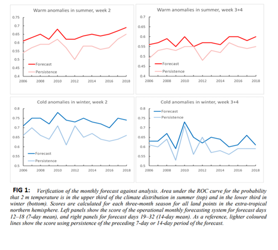
Monthly forecast verification statistics and performance (Figure 1) shows the probabilistic performance of the monthly forecast over the extratropical northern hemisphere for summer (JJA, top panels) and winter (DJF, bottom panels) seasons since September 2004 for week 2 (days 12–18, left panels) and week 3+4 (days 19–32 right panels). Forecast skill for week 2 exceeds that of persistence by about 10%, for weeks 3 to 4 (combined) by about 5%. In weeks 3 to 4 (14-day period), summer warm anomalies appear to have slightly higher predictability than winter cold anomalies, although the latter has increased in recent winters (with the exception of 2012). (Source: ECMWF)
In 2018, week 2 forecast skill for summer warm anomalies was unusually high, but persistence was also at its highest level within the period shown. The corresponding week 3+4 forecast skill and persistence were also near the upper end of values seen so far. Skill for winter cold anomalies in 2018 was close to average, however in week 2 there is an increasingly consistent margin relative to persistence in recent years.
SEASONAL FORECASTS ARE NOT WEATHER FORECASTS: THE ROLE OF THE HINDCASTS
Seasonal forecasts are started from an observed state of (all components of) the climate system, which is then evolved in time over a period of a few months. Errors present at the start of the forecast (due to the imprecise measurement of the initial conditions and the approximations assumed in the formulation of the models) persist or, more often, grow through the model integration, reaching magnitudes comparable to that of the predictable signals. Some such errors are random; the effect of these on the outcome is quantified through the use of ensembles. Some errors, however, are systematic; if these systematic errors were determined, corrections could be applied to the forecasts to extract the useful information. This is achieved by comparing retrospective forecasts (reforecasts or hindcasts) with observations. The same forecast system is run for several starting points in the past in the same way as a forecast would be run (with only knowledge of the starting point), for the same length of time as an equivalent forecast. The resulting data set constitutes a ‘climate’ of the model, which can then be compared with the observed climate of the real world. The systematic differences between the model and the real world – usually referred to as biases – are thus quantified and used as the basis for corrections which can be applied to future, real-time forecasts. Given the relative magnitude of such biases, some basic corrections are essential to convert the data into forecast information – therefore a forecast by it-self is not useful without relating it to the relevant hindcasts.
Fig 2 below is an example of the crucial role of the hindcasts in seasonal forecasting. It shows the time evolution of monthly-average temperature in a given region, between May and December: the blue line represents the average conditions observed over a period in the past
(the reference period; in this case, 1993-2014), the red line is the equivalent model climate average over the same reference period. The difference between the two clearly indicates a significant cold bias, increasing with the time into the forecast. An ensemble of forecasts for a particular year is shown as green lines. When compared to the observed ‘normal’, all green ensemble pre-dictions are for colder-than-normal conditions – not necessarily surprising when remembering that the model is systematically colder than the real world. However, when comparison is made with the model’s ‘normal’ (the red line), all forecast ensemble members indicate warmer-than-normal conditions. Clearly as the forecast is an output of the model, the latter comparison is the more appropriate.
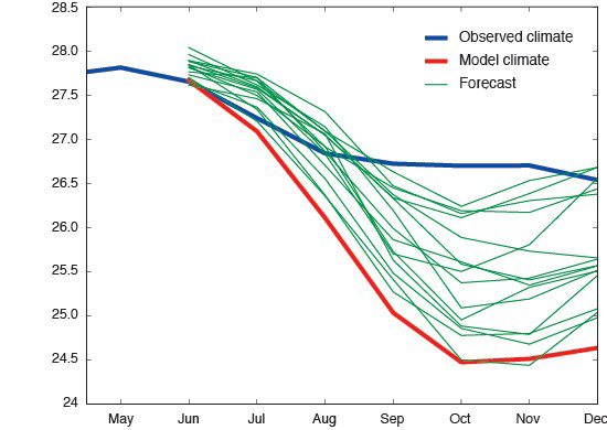
Fig 2: The time evolution of monthly-average temperature in a given region, between May and December
As well as playing an essential role in the correction of systematic errors, hindcasts are also used to assess the skill of seasonal forecast systems (by comparing each of the forecasts for the years in the reference period with the respective observed conditions). Information on forecast skill is important to avoid overconfident decision making.
Note that for reasons related with the availability of computing resources, the hindcasts usually have fewer ensemble members per start date than the real-time forecasts, e.g. ECMWF SEAS5 5 has 51 members for the real-time forecasts, and just 25 members for the hindcasts.(Source: ECMWF).
For further details and plots on the verification of seasonal forecast, data provided by C3S please visit https://confluence.ecmwf.int/display/CKB/C3S+seasonal+forecasts+verification+plots
VERIFICATION TOOLS AND VERIFICATION SKILL SCORES OF THE ECMWF MONTHLY FORECASTING SYSTEM
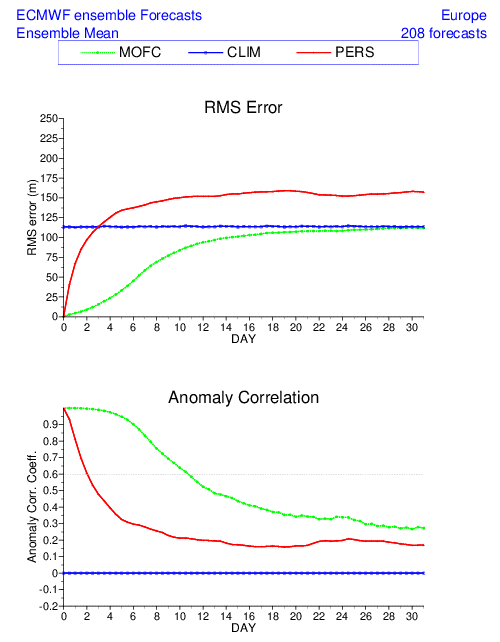
Fig 3: A comparison of the RMSE and Anomaly Correlation of the monthly forecasting system (MOFC) over Europe against climatology (CLIM) and persistence (PERS). Scores are computed from forecasts on a standard 2.5° x 2.5° grid limited to standard domains. The bottom panel displays the anomaly correlation score of daily monthly forecasts of 500 hPa geopotential height over several regions. Anomaly correlation scores are spatial correlation between the forecast anomaly and the verifying analysis anomaly. The top panel displays
the Root Mean Square Errors (RMSE) of daily monthly forecasts of 500 hPa geopotential height over several regions. Root Mean Square Errors are the geographical average of the squared differences between the forecast and the analysis valid for the same time (Source: ECMWF).
- The ECMWF Monthly Forecast System root mean square error (RMSE) is lower than the persistence RMSE throughout the forecast period whilst is notably lower than the climatology RMSE through until day 16, thereafter it is similar to climatology but with a slightly smaller error.
- The Anomaly Correlation of the ECMWF Monthly Forecast System is higher than both climatology and persistence through to Day 30.
For further details on the verification of monthly forecast data provided by the ECMWF and analysed by Meteorologists at Met Éireann please visit: https://www.ecmwf.int/en/forecasts/quality-our-forecasts
CASE STUDY: EUROPEAN COLD SPELL FEBRUARY 2018
A particular case when the sub-seasonal forecast proved very useful was ahead of the severe cold spell in Europe in late February 2018. Below we can see the evolution of the forecast from as early as 1 February and compare with the analysed temperature and pressure anomalies. We can see cold anomalies over Europe began to be heralded in early February. In this instance the forecaster had growing confidence that there was a risk of exceptional cold weather in the region in late February.
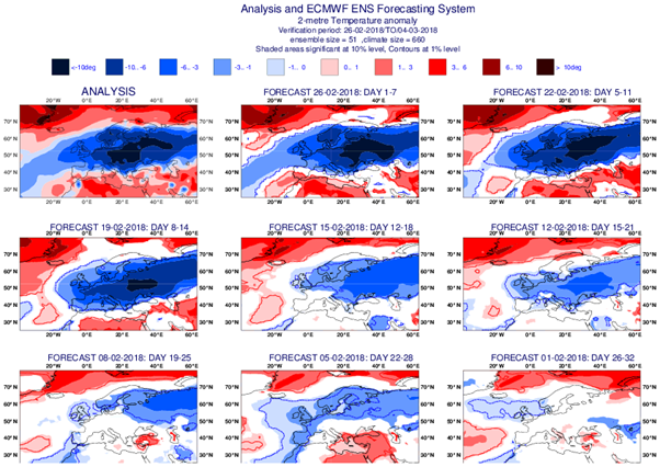
(Fig 4: Analysis and ECWMF ENS Forecasting system 2-metre temperature anomaly for week 26-02-2018 to 04-03-2018)
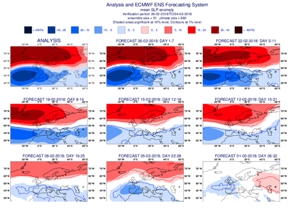
(Fig 5: Analysis and ECWMF ENS Forecasting system MSLP anomaly for week 26-02-2018 to 04-03-2018)
Fig 4-5: These graphics displays the weekly mean anomalies relative to the past 20-year climate. The first panel corresponds to the anomalies computed using ECMWF operational analysis and reanalysis for a given week. The other panels correspond to the eight monthly forecasts starting one week apart and verifying on that week. The model anomalies are relative to the model climate computed from the model back-statistics. The areas where the ensemble forecast is not significantly different from the ensemble climatology according to WMW-test are blanked. The time range of the forecasts is day 1-7, day 5-11, day 8-14, day 12-18, day 15-21, day 19-25, day 22-28 and day 26-32. This figure gives an idea of how well the predicted anomalies verified against the ECMWF analysis and also about the consistency between the monthly forecasts from one week to another (Source: ECMWF).